This page continues the Guide of the Modeling Fairy App. The app builds the models and shows their volumes and Bayes factors; the program QTest (Zwilling et al. (2019); Regenwetter et al. (2014)) adds the frequentist tests and the Bayesian p value. The walkthrough uses the same made-up data and the first model of the Guide.
Preparation
Before we start the actual analysis, we need to first download and install QTest. Download links for both the Mac and Windows operating systems are available on the website here.
Of the many analyses that the Shiny app provides, the \({\cal H}\)-representation is key to running statistical analyses in QTest. Now that we have obtained the \({\cal H}\)-representations for all models using the fairy app, we will walk through how to test our hypotheses using QTest and how to view the results. As a demonstration, we will take a look at how much evidence the made-up data presented in Table 1 provide against, or in support of, the first hypothesis as formalized in model m1 of the Guide (cringyness increases with age).
| Cringe at illogical jokes | No Cringe at illogical jokes | Cringe at puns | No Cringe at puns | |
|---|---|---|---|---|
| Children | 60 | 40 | 60 | 40 |
| Teens | 64 | 36 | 50 | 50 |
| Adult | 68 | 32 | 38 | 62 |
Next, recall that, under the “\({\cal H}\)-representation” tab in the Shiny app, we can download the file that contains the \({\cal H}\)-representation of our model of interest in a tar-archive file. Before we start our analysis, we extract the text file that contains the \({\cal H}\)-representation of m1. You can also download the file created by the fairy app for Model 1 here, all models reported in the article are also included on the OSF-website here.
We also need to make sure that the constraints in the \({\cal H}\)-representation and the way in which we communicate the empirical data to QTest are properly aligned. (The same applies to any \({\cal V}\)-representation when communicating that to QTest.) To this end we will create labels for all possible types of observations. For instance, we may observe that a child cringes at the pun. We may observe that a teen does not cringe at the illogical joke. In the manuscript, there are 3 x 2 x 2 = 12 different types of observations: Children, teens, and adults (3 cases) may cringe or not cringe (2 possible responses) at the pun or the illogical joke (2 cases). We will use
- “A” to denote that a child cringes at the illogical joke,
- “B” to denote that a child does not cringe at the illogical joke,
- “C” to denote that a teen cringes at the illogical joke,
- “D” to denote that a teen does not cringe at the illogical joke,
- “E” to denote that an adult cringes at the illogical joke,
- “F” to denote that an adult does not cringe at the illogical joke,
- “G” to denote that a child cringes at the pun,
- “H” to denote that a child does not cringe at the pun,
- “I” to denote that a teen cringes at the pun,
- “J” to denote that a teen does not cringe at the pun,
- “K” to denote that an adult cringes at the pun,
- “L” to denote that an adult does not cringe at the pun.
Note that QTest only uses letter labels: The user needs to keep track of their meanings separately.
Setting dimensions / Coordinates
After opening up QTest, we need to first specify the number and names of parameters that the models use, in a fashion consistent with how we coded the order-constraints. We enter this information in the “Gamble pairs” panel that is located in the top left of the interface.
To create the correct number of parameters, QTest requires that we first indicate a number of “gambles.” The original QTest interface was designed for decision making research. Here, think of each “gamble” as a label for a possible type of observation. In the preparatory work above, we ear-marked 12 labels. Having specified that we need 12 labels, if we click on “Set…”, we see that QTest provides a huge list of possible label pairs. This step defines the Binomial parameters that we use in our models.
The labeling must be consistent with the \({\cal H}\)-representation. In this list, we select the 6 pairs that correspond to the six Binomials that we are interested in: The appropriate labels for the 6 Binomial parameters are therefore “(A,B),” “(C,D),” “(E,F),” “(G,H),” “(I,J),” and “(K,L)”.
Among these, for instance “(I,J)” denotes the Binomial process for teens and puns, in which “I” denotes the outcome that the teen cringes at the pun, whereas “J” denotes the outcome that the teen does not cringe at the pun.
All the steps just explained for setting up the dimensions are illustrated in the following video.
We must ensure that we do not accidentally code the Binomials in opposite ways between the Shiny app and QTest: Say, if p1 denoted the probability of “cringing” in the Shiny app, but “A” denoted “not cringing” in QTest whereas “B” denoted “cringing,” then the QTest coordinate system would mismatch that in the Shiny app and the resulting QTest analyses would be wrong because the data and/or order-constraints would be coded incorrectly in QTest.
Loading Data
To input the empirical data, we navigate to the “Data” panel in the lower left corner of the GUI. There are two methods for entering data. The first method is to input the data manually using the “Enter” button. You can see all the steps in the video clip below. To learn how to load data from a file and how to load multiple data sets, refer to the general-purpose QTest tutorial available for download here.
When manually entering data in QTest, you have two options:
- Using a Preset Sample Size: If you set the “Sample size N” to some value, you only need to enter the first value for each coordinate. QTest will automatically calculate the second. For instance, if you set the preset “Sample size N” to 100 and enter 60 for A, QTest will automatically fill in 40 for B.
- Entering All Data Manually: If your sample size varies between Binomials, you can enter all observations by hand and ignore the “Sample size N” option. QTest will later display the range of sample sizes based on your input.
We use the preset option in the tutorial, as shown in the next video. ]{.aside}
We recommend that you verify whether you coded the data consistently with the coordinate system you created earlier. In the video clip above, the “Data” section shows that “A” was observed 60 times, “B” 40 times, “C” 64 times, and “L” 62 times.
Loading a Model
To load a model into the software, we move to the “Probabilistic specifications” panel that is located to the right of the “Data” panel.
The QTest GUI offers three types of specifications, all of them labeled for use in decision making research. We use what QTest calls the “Random preference” specification, as a backdoor. We load Model 1 by clicking on the “Load” button and selecting the “m1.txt” file in the pop-up window.
All the steps for loading Model 1 are illustrated in the following video.
Like above for the data, it is a good idea to cross-check that the order-constraints in the txt file are also aligned with the coding of our coordinate system in QTest to ensure that we do not end up running nonsensical analyses. To that end, we cross-check the Shiny app constraints that we exported as a QTest compatible machine readable file. The first probability (\(p_1\)) is the probability that a child cringes at the pun. The first Binomial parameter in the “Gamble pairs” panel of QTest is “(A,B),” where “A” is the event that a child cringes at the illogical joke. Since p1 is indeed the probability of observing “A,” and 1-p1 is indeed the probability of observing “B,” we have perfect alignment between the first coordinate in QTest and the first parameter in the Shiny app. It is worthwhile to cross-check each of the parameters in QTest against each of the parameters in the Shiny app to make sure that we communicated the information correctly from the Shiny app to QTest.
Analysis
We next move to the “Hypothesis testing” panel to demonstrate how we can run different analyses in QTest. Right beneath the “Run test” button, there are three panels. Since we are only examining one hypothesis at a time, we leave the “Theories” and “Specifications” panels at their default settings. Since we are only looking at a single dataset, we can also leave the “Data sets” panel at the default setting. If we wanted to look at multiple data sets, then we could choose the option “All” for “Data sets.”
In the next panel, we choose which type of analysis we want to run (QTest calls this the “Type of test”). Note, we advise against choosing the “all” option because different types of analyses require different settings for optimal performance.
To compute a frequentist \(p\)-value, choose the “Frequentist” option. Then click on the “Run test” button at the top of the “Hypothesis testing” panel to run the analysis.
There is no (algorithm for) a frequentist test of an order-constrained model that is not full-dimensional (Davis-Stober, 2009). Here, Models 5 (all six probabilities equal) and 6 (equal averages) are one-, respectively five-dimensional. Hence, QTest cannot run a frequentist test. However, since Model 5 is not order-constrained, it can be tested using standard tools outside of QTest.
To compute a Bayesian \(p\) value, choose the “Bayes \(p\) & DIC” option in the “Type of test” panel. Before launching the analysis, we further adjust some options immediately beneath to customize our analysis. Since QTest uses two (distinct) Gibbs sampling algorithms to calculate Bayes \(p\) and Bayes factors, we need to indicate the number of samples, the burn-in size, and a random seed for the pertinent Gibbs sampler. The number of draws is relevant to all users, whereas only advanced users need to worry about changing the burn-in size from its default. The random seed is useful for all users. We will talk about it below when we discuss how to assess convergence of a Gibbs sampling algorithm. We recommend starting with a “Sample size” of 100,000 draws and then scaling up if the estimates of the Bayes \(p\) is not converging. We discuss how to assess convergence in the next section. In our example, we draw 100,000 samples and use 1,000 as the burn-in size. To select a sample size for the Gibbs Sampler, click on the “Change” button next to “Sample size:” and input, for instance, “100000.” (To change the burn-in size, follow the analogous steps.)
To compute Bayes factors, the users choose the “Bayes factor” option in the “Type of test” section. Similar to the Bayes \(p\) analysis, we can also adjust the sample size for the Gibbs sampler algorithm, the burn-in size, and the random seed number. To indicate the sample size you would like to use, click on the “Change” button next to “Sample size,” and input your preferred value. A reasonable number here would be 1,000,000. (Advanced users can change the burn-in size similarly.) After you are done with your customization, click on the “Run test” button at the top of the “Hypothesis testing” panel to run the analysis.
The following video demonstrates all the steps for setting up the analysis as explained above. Please note that we edited the video to keep it brief.
Before we investigate the results, there is one more important point to address. Because order-constrained analytics utilize Monte Carlo simulation methods, a user should assess convergence for all results to ensure that the estimates are sufficiently accurate. This usually only affects Bayesian \(p\) value and Bayes factor computations. We consider, for brevity, the latter next.
One way to check whether our estimates of the Bayes factor have converged is to run the same analysis using two or more different random seeds. To change the seed you are using for the analysis, click on the “Set” button in the “Random number seed” panel. As a demonstration in the next video, we input “2” as our second random seed. Below, we will compare the results from the two different seeds to see whether the Bayes factors are substantially different. The differences give us a gauge of how well the algorithms have converged to an accurate result.
We can view the results from our analyses in the “Results” table located at the bottom of the “Hypothesis testing” panel. To view a summary table with results from all of your analyses, click on the “Table” button. To examine results from a single analysis in detail, first select the analysis by clicking on it, then click the “Details” button.
The following video demonstrates all the steps for conducting a repeated analysis and examining all the results.
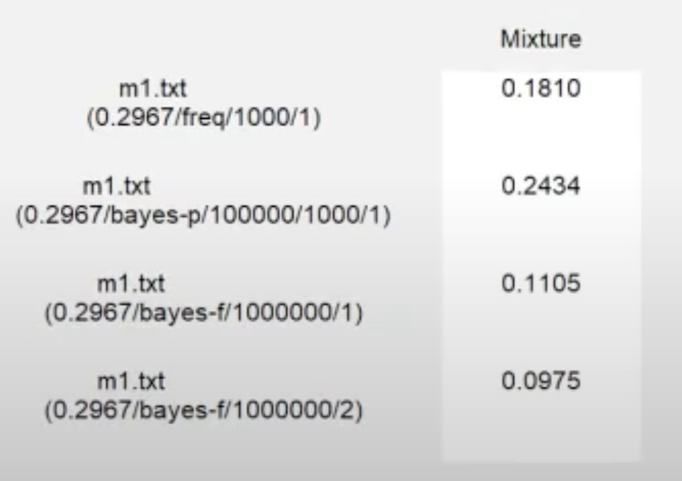
Looking at the results from the analysis as displayed below, we see that the frequentist \(p\)-value is 0.1810. A frequentist \(p\)-value of 0.1810 (since it exceeds \(\alpha =0.05\)) suggests an adequate fit of m1 on the data. The Bayesian \(p\) value is 0.2434. A Bayesian \(p\) value of 0.2434 (since it exceeds \(0.05\)) indicates an adequate fit of m1 on the data.
Looking at the details from the multiple Bayes factor analyses, we see that the Bayes factor estimate from the first seed is 0.1105 and the Bayes factor estimate from the second seed is 0.0975. A Bayes factor around \(0.1 \pm 0.02\) would indicate that, despite the adequate fit of the model when viewed through the frequentist and Bayesian \(p\) values, we have “substantial” or “strong” evidence against m1 in comparison to the unconstrained model (Jeffreys, 1998) when weighing fit against parsimony.
If the range \(0.1 \pm 0.02\) is correct, the conclusion that this model is not viable does not depend on obtaining a higher level of precision for the Bayes factor estimate. Depending on the situation, it may, therefore, not be critically important to invest more computing power and time into achieving higher precision for this Bayes factor (but see below).
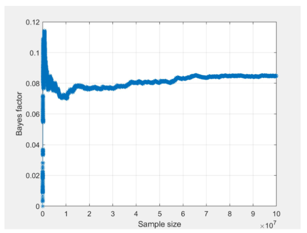
Another useful tool to examine convergence of Bayes factor estimates is the “convergence plot” as displayed below for seed 1 and 2. After selecting a Bayes factor analysis in the lower right panel, click on the “Details” button underneath the table of results to view details about the analysis and the corresponding convergence plot. The horizontal axis is the cumulative sample size of the Gibbs sampler, which is effectively the same as computation time flowing from left to right. The vertical axis is the estimate of the Bayes factor at that time point.
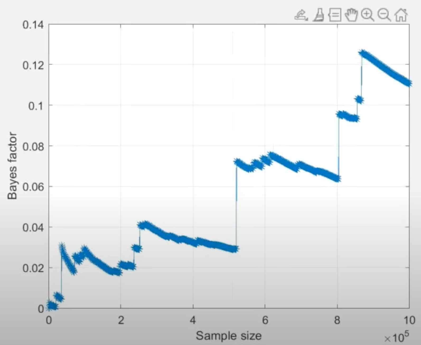
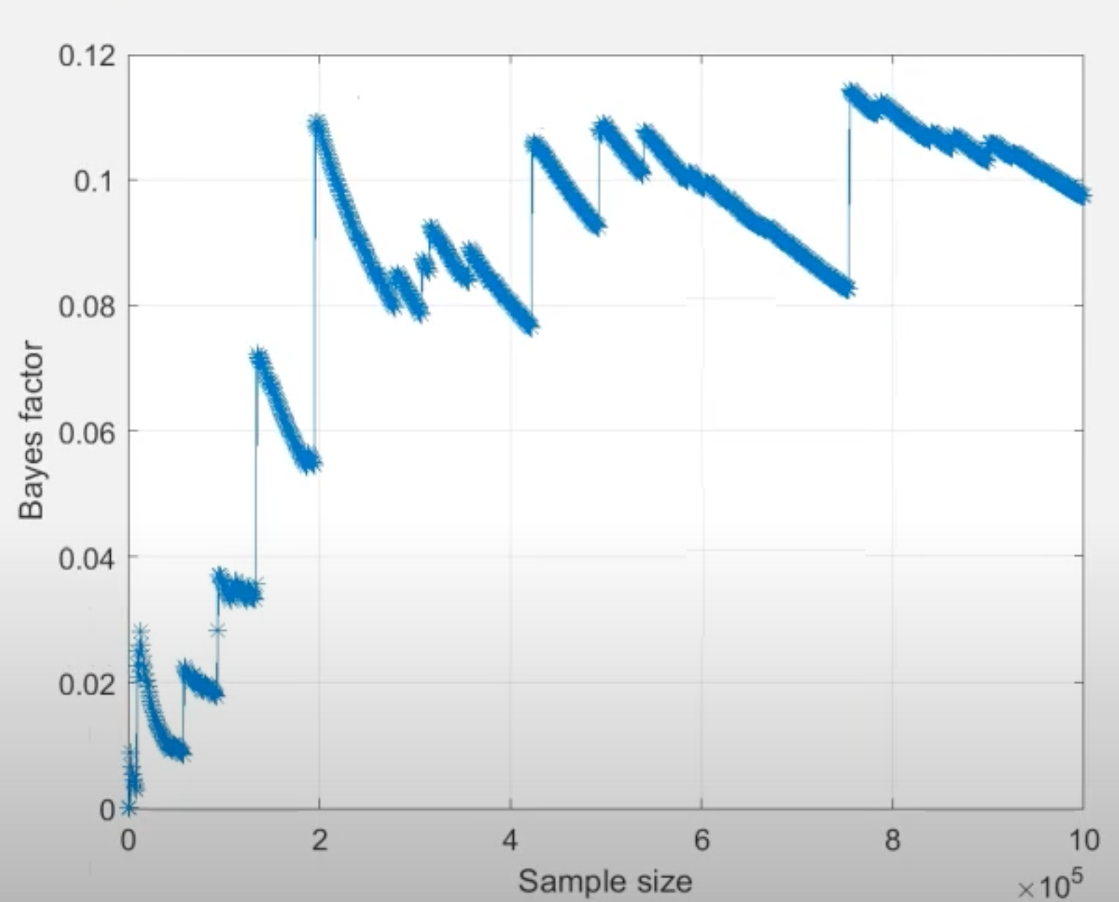
Based on the “jumps” displayed towards the end of both convergence plots, we conclude that the Bayes factor estimate has remained unstable throughout the computation, hence it has not converged. For convergence, we would need to increase the number of draws until we see a smooth horizontal trend in the right side of the convergence plot.1
1 A horizontal convergence plot is a prerequisite, but not a guarantee of convergence. We recommend consulting with tutorial resources (e.g., Regenwetter, 2020; Regenwetter & Cavagnaro, 2019; Regenwetter & Robinson, 2019, for order-constrained analytics) on how to determine what constitutes sufficiently good evidence of convergence of an approximation algorithm.
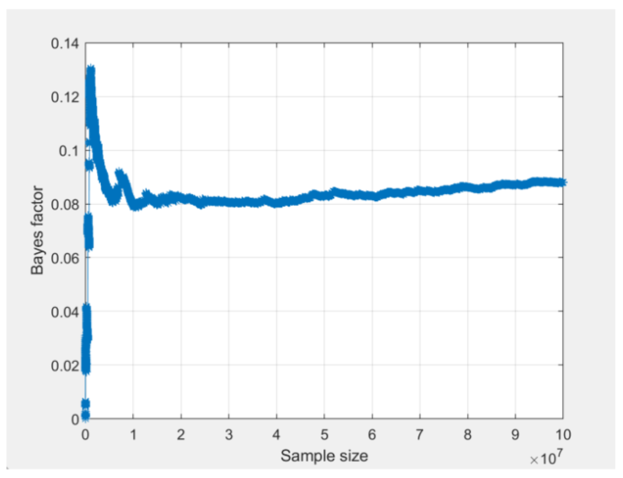
To get results with better convergence, we increase the draw size to 100,000,000 draws. The screenshot below shows the convergence plots for m1 from the two different seeds, after increasing the draw size to 100,000,000 (notice that the vertical axis in the two QTest convergence plots is scaled slightly differently). In contrast to the convergence plots presented above, these convergence plots have smooth horizontal trends on the right side.
The lack of “jumps” towards the end of the plots show that the estimate of the Bayes factor has stabilized. Furthermore, when we compare the two convergence plots, we can see that they both stabilize around the same time and are trending towards the same value between 0.08 and 0.09. The actual value of the Bayes factor for both runs can be viewed by clicking the “Table…” button as demonstrated in the last video.
Although we could invest more computing power to reach more precise convergence, this would not change our conclusion that this model is not viable. Thus, we are satisfied with this level of convergence and report our results to the nearest converged decimal place.
For your convenience, to quickly re-run the analysis without going through the steps of preparation, setting dimensions, and loading data, you can load this file in QTest by pressing “Load” in the “File” section below the visualization section as demonstrated in the final video.
Back to the Guide. The Guide shows how to enter the models, how to read their volumes, and how to run the Bayesian analysis with multinomineq in the app: Modeling Fairy App, Guide.