From a verbal theory to a testable model
This guide follows the fictitious cringe study of the article, from three probabilities to nine theories, their overlap, their volumes, and a first Bayesian analysis of data. Each step has a short animation of the app and the explanation next to it.
You can do everything hands-on: in the app, click Take a tour and choose The cringe study. The pointer enters everything for you, or you switch to Try it yourself and type it in.
Prefer to watch? The whole guide as one narrated video
About 22 minutes, recorded from the app and narrated in English; waiting times are sped up. Switch the captions on and off with the button below the video, and click a chapter to jump there. Download the video (25 MB)
The cringe study
Does a joke make you cringe? That depends on who you are, and on the joke.
In the article (Jekel et al., in revision) we run a fictitious joke study. Children, teens and adults hear either illogical jokes or puns (a 2 x 3 design), and in every condition we observe the proportion of people who cringe. Nine cringe theories predict how these proportions relate. The app turns each theory into a model: a set of constraints on the proportions, which it can then draw, measure and test.
The proportion of people who cringe in a condition is a probability. We write \(p_C\), \(p_T\) and \(p_A\) for children, teens and adults. In a model they are always called p1, p2, p3, … in the order of the name fields at the top of the app; the names are only labels.
How to use this guide. The animations show the app while the pointer works; the text next to them says what happens and why. Boxes titled Input for the app contain text you can copy into the field Unique Model Specification. The app also has a tour that does all of this for you: Take a tour, then The cringe study. We start with a simpler example than the article, to introduce the central ideas.
A first model: three age groups
Three probabilities, one theory, one click on Go.
Our first theory says that children cringe at least as much as teens, who cringe at least as much as adults:
\[p_{C} \geq p_{T} \geq p_{A}\]
In the app you first name the three probabilities (the fields at the top, for example p_{C}, p_{T} and p_{A}), then you type the theory into the field Unique Model Specification. There you refer to the probabilities by their numbers.
p1 > p2 > p3The app asks for > as an easier-to-type symbol; it means “at least as much as”, exactly the \(\geq\) of the theory. p1 is the probability whose name sits in the field Name of p1, and so on.
Optionally the app also computes the vertices of the model (corner points, see the next section). They are switched on per model with the V button next to the model, because they can take long for large models. Then Go builds the model: the app needs a moment, and the result tabs H-representation, V-representation, Plot Edge Cases, Plot Polytope(s) and Parsimony appear next to Input.
H- and V-representation: two ways to describe a model
Inequalities describe what the theory allows, corner points show its extreme cases.
H-representation
The H-representation is a minimal description of your theory by inequalities. The app uses an R package (Geyer & Meeden, 2023) to compute it. For the first model the result is short:
- The first line says that \(p_2 \leq p_1\): the second probability is at most the first.
- The second line says that \(p_3 \leq p_2\).
- The third line says that \(p_1 \leq 1\), and the fourth line that \(0 \leq p_3\). These two are automatic: probabilities lie between 0 and 1.
On the left side of the app you can download the H-representation as files for QTEST (Zwilling et al., 2019; Regenwetter et al., 2014) or for the R package multinomineq, and as a LaTeX file ready for compilation.
The polytope
With three probabilities a model is a body inside a cube. Each axis is one probability from 0 to 1, so the cube holds all possible triples. The coloured figure marks the triples that fit your theory; the triples outside do not. Such a figure is called a polytope. You can rotate it with the mouse.
V-representation
A polytope is also described by its corner points, the vertices. For the first model there are four: \(V_1 = (1,1,1)\), \(V_2 = (1,1,0)\), \(V_3 = (1,0,0)\) and \(V_4 = (0,0,0)\). The tab V-representation lists them as a matrix: one row per vertex, one column per probability. Vertices are valuable because they are the edge cases of the theory: the most extreme patterns it still allows. The tab Plot Edge Cases steps through them.
When to switch the vertices on. For most analyses the H-representation is enough, and QTEST and multinomineq can work with it. Vertices can become very costly: as a rule of thumb, avoid them for models with more than about fifteen probabilities.
How restrictive is a theory? Volume and maximum Bayes factor
A theory that forbids more can earn more evidence, and risks more.
Seeing a model as a polytope lets us measure parsimony, a usually vague idea: the smaller the polytope, the more the theory forbids. This is close to Popper’s criterion of empirical content (Glöckner & Betsch, 2011; Popper, 1934/2005). In the tab Parsimony, Go computes the volume of every model, that is the share of the cube that fits the theory. The app uses an R package (Fisikopoulos & Chalkis, 2023) and an exact method where possible.
For p1 > p2 > p3 the volume is 1/6, about 17 percent: three numbers can be ordered in six ways, and only one of them fits.
The volume is also linked to Bayesian analysis. The reciprocal of the volume, here 6, is the largest possible Bayes factor the theory can reach against an unconstrained model in which the probabilities can take any value. The tighter a theory is, the more evidence it can earn, and the more it risks. If the largest possible Bayes factor is too low for your purposes, revisit the stimuli to find conditions in which your theory forbids more; this is closely related to optimal study design (Myung & Pitt, 2009).
Volumes of algorithms that estimate can vary a little between runs; the app shows the volume for each algorithm you choose and lets you tighten the approximation error. The results can be downloaded as a csv table.
The full study: six probabilities and nine theories
Now the study of the article, in the app and in your own copy-and-paste.
In the full study we add a second factor: the joke is either illogical or a pun. We mark illogical jokes with \(\looparrowright\) and puns with \(\heartsuit\) (because we love puns). With a 2 x 3 design we have six probabilities:
- \(P^\looparrowright_C\) = p1: a randomly drawn child cringes at an illogical joke.
- \(P^\looparrowright_T\) = p2: a teen cringes at an illogical joke.
- \(P^\looparrowright_A\) = p3: an adult cringes at an illogical joke.
- \(P^\heartsuit_C\) = p4: a child cringes at a pun.
- \(P^\heartsuit_T\) = p5: a teen cringes at a pun.
- \(P^\heartsuit_A\) = p6: an adult cringes at a pun.
You add three probabilities with the + button next to Probabilities, name all six, and add eight more model rows with the + button next to Model(s). Then you can type the nine theories.
The nine theories
Click a theory to see what it says and which text to type. All inputs can be copied. Or you open the app with all nine theories already entered, with the six names and the settings: open the app with all nine models. The link opens the page with the app tab, the input is restored there.
| Model | In words |
|---|---|
| m1 | cringyness increases with age (averaged over both joke types) |
| m2 | cringyness increases with age for each joke type |
| m3 | opposite trends; illogical jokes on average less cringy than puns |
| m4 | like m3, and puns are cringier in every age group |
| m5 | both joke types exactly equally cringy in all age groups |
| m6 | the trends balance out: equal averages |
| m7 | like m6, with the averages allowed to differ by .05 |
| m8 | all six probabilities about the same, within .05 |
| m9 | the opposite of m4 |
The nine theories in detail
Each card below is one theory. Click a card to open it: it says in words what the theory predicts, shows the formula from the article, and gives the text to type into the field Unique Model Specification (the copy button is at the right end of the box).
Cringyness increases with age, averaged over both joke types:
\[\underbrace{\frac{P^\looparrowright_C + P^\heartsuit_C}{2}}_{\mbox{children}} \leq \underbrace{\frac{P^\looparrowright_T +P^\heartsuit_T}{2}}_{\mbox{teens}} \leq \underbrace{\frac{P^\looparrowright_A +P^\heartsuit_A}{2}}_{\mbox{adults}}.\]
Input for the app:
1/2 * p1 + 1/2 * p4 < 1/2 * p2 + 1/2 * p5 < 1/2 * p3 + 1/2 * p6Sums with weights are typed as 1/2 * p1. Long input can be enlarged with the arrows in the corner of the field.
\[\underbrace{P^\looparrowright_C \leq P^\looparrowright_T \leq P^\looparrowright_A}_{\mbox{illogical jokes}} \;\; \mbox{and} \;\; \underbrace{P^\heartsuit_C \leq P^\heartsuit_T \leq P^\heartsuit_A}_{\mbox{puns}}.\]
Input for the app:
p1 < p2 < p3; p4 < p5 < p6Two chains, separated by a semicolon.
Cringyness decreases with age for illogical jokes and increases with age for puns, and illogical jokes are on average less cringy than puns:
\[P^\looparrowright_C \geq P^\looparrowright_T \geq P^\looparrowright_A \;\; \mbox{and} \;\; P^\heartsuit_C \leq P^\heartsuit_T \leq P^\heartsuit_A, \;\; \mbox{and} \;\; \frac{P^\looparrowright_C + P^\looparrowright_T + P^\looparrowright_A}{3} \leq \frac{P^\heartsuit_C + P^\heartsuit_T + P^\heartsuit_A}{3}.\]
Input for the app:
p1 > p2 > p3; p4 < p5 < p6; 1/3 * p1 + 1/3 * p2 + 1/3 * p3 < 1/3 * p4 + 1/3 * p5 + 1/3 * p6Like m3, but puns are cringier than illogical jokes in every single age group:
\[P^\looparrowright_C \geq P^\looparrowright_T \geq P^\looparrowright_A, \;\; P^\heartsuit_C \leq P^\heartsuit_T \leq P^\heartsuit_A, \;\; P^\looparrowright_C \leq P^\heartsuit_C, \;\; P^\looparrowright_T \leq P^\heartsuit_T, \;\; P^\looparrowright_A \leq P^\heartsuit_A.\]
Input for the app:
p1 > p2 > p3; p4 < p5 < p6; p1 < p4; p2 < p5; p3 < p6Both joke types are exactly equally cringe-worthy in all three age groups:
\[P^\looparrowright_A = P^\heartsuit_A = P^\looparrowright_T = P^\heartsuit_T = P^\looparrowright_C = P^\heartsuit_C.\]
Input for the app:
p1 = p2 = p3 = p4 = p5 = p6A model with exact equalities has volume zero, so there is no upper limit for the Bayes factor in its favour.
Cringyness decreases with age for illogical jokes and increases for puns, but the two balance each other out: overall, puns are exactly as cringy as illogical jokes:
\[P^\looparrowright_C \geq P^\looparrowright_T \geq P^\looparrowright_A \;\mbox{and}\; P^\heartsuit_C \leq P^\heartsuit_T \leq P^\heartsuit_A, \;\mbox{and}\; \frac{P^\looparrowright_C + P^\looparrowright_T + P^\looparrowright_A}{3} = \frac{P^\heartsuit_C + P^\heartsuit_T + P^\heartsuit_A}{3}.\]
Input for the app:
p1 > p2 > p3; p4 < p5 < p6; 1/3 * p1 + 1/3 * p2 + 1/3 * p3 = 1/3 * p4 + 1/3 * p5 + 1/3 * p6m7 reads “about equally cringy” differently: the averages of both joke types do not have to be exactly equal, they may deviate by .05:
\[P^\looparrowright_C \geq P^\looparrowright_T \geq P^\looparrowright_A \;\mbox{and}\; P^\heartsuit_C \leq P^\heartsuit_T \leq P^\heartsuit_A, \;\mbox{and}\; \left| \frac{P^\looparrowright_A + P^\looparrowright_T + P^\looparrowright_C}{3} - \frac{P^\heartsuit_A + P^\heartsuit_T + P^\heartsuit_C}{3} \right| \leq 0.05.\]
Input for the app: the same as for m6.
Then the equality is switched to an approximate one with the button Approximate equalities in the row of m7, with the tolerance .05.
All six probabilities are about the same, as in m5, but with a wiggle room of .05 for every pair:
\[|p_i - p_j| \leq 0.05, \;\; \mbox{for each distinct pair } p_i, p_j.\]
Input for the app:
{p1,p2,p3,p4,p5,p6} = {p1,p2,p3,p4,p5,p6}The braces are a shortcut for p1 = p2; p1 = p3; …; p5 = p6: every element on the left is set equal to every element on the right (pairs such as p1 = p1 are removed). Then the equalities are switched to approximate with the tolerance .05.
\[P^\looparrowright_C \leq P^\looparrowright_T \leq P^\looparrowright_A, \;\; P^\heartsuit_C \geq P^\heartsuit_T \geq P^\heartsuit_A, \;\; P^\looparrowright_C \geq P^\heartsuit_C, \;\; P^\looparrowright_T \geq P^\heartsuit_T, \;\; P^\looparrowright_A \geq P^\heartsuit_A.\]
Input for the app:
p1 < p2 < p3; p4 > p5 > p6; p1 > p4; p2 > p5; p3 > p6Model 10 of the article cannot be created easily with the current version of the app. H- and V-representations of all models are provided on the OSF page of the project.
What theories share: intersections
Two theories can predict similar things. Their polytopes then overlap.
How much two theories share can be seen geometrically: the intersection of two polytopes is the space both contain. The button Intersection model adds a row with all constraints of the models you tick. Written as input, the intersection of m1 and m2 is simply all their constraints together:
1/2 * p1 + 1/2 * p4 < 1/2 * p2 + 1/2 * p5 < 1/2 * p3 + 1/2 * p6; p1 < p2 < p3; p4 < p5 < p6The volume of the intersection of m1 and m2 is as large as the volume of m2. So m1 completely overlaps m2: m2 is nested in m1. Whenever data fit m2 they also fit m1. Because m2 is smaller it earns more evidence in a Bayesian analysis, and it is preferred for parsimony.
The intersection of m1 and m3 is different: they overlap, but not completely. The two theories predict distinctly different outcomes, which is what you want. If the overlap is too large, consider other stimuli. The intersection of m4 and m9 has volume zero: the surfaces of both models only touch, in the points where all six probabilities are equal.
1/2 * p1 + 1/2 * p4 < 1/2 * p2 + 1/2 * p5 < 1/2 * p3 + 1/2 * p6; p1 > p2 > p3; p4 < p5 < p6; 1/3 * p1 + 1/3 * p2 + 1/3 * p3 < 1/3 * p4 + 1/3 * p5 + 1/3 * p6Results for all models
One card per model, and the volumes side by side.
Go builds all models at once. In the tab H-representation every model has its own card; the badge counts equalities and inequalities (the five equalities of m5 show up as “5 eq”). A card can be enlarged with the arrows in its corner, and cards can be arranged: the compact view packs the terms of a row together, hide the trivial bounds leaves only what is specific to the model, and the free layout lets you drag a card anywhere. The circle arrow puts everything back.
Under Parsimony the bars compare the volumes of all models, including the intersections. The table lists the largest possible Bayes factor of every model: tighter models can earn more evidence, and risk more. Models with an exact equality have volume zero, so there is no upper bound.
A first analysis with data
So far the theories were compared by what they allow. Now they meet data.
We use made-up data: one hundred children, teens and adults each answered for both joke types.
| Cringe at illogical jokes | No cringe at illogical jokes | Cringe at puns | No cringe at puns | |
|---|---|---|---|---|
| Children | 60 | 40 | 60 | 40 |
| Teens | 64 | 36 | 50 | 50 |
| Adults | 68 | 32 | 38 | 62 |
The Data window of the analysis takes the numbers. For every probability it asks for n, the number of observed cases, and the frequency, how often the cringe happened. Here n is 100 for every row (the field Same n for every row sets them all), and the frequencies are 60, 64, 68, 60, 50 and 38 for p1 to p6. Save keeps them for the analysis and for the downloads.
Run analysis starts the Bayesian analysis of all models with the R package multinomineq (Heck & Davis-Stober, 2019). It runs on a shared server, so it is meant for smaller analyses; larger analyses can be run on your own computer with the R script of the download. The setting Samples is the number of random draws. With the standard 10,000 draws a theory the data contradict strongly gets only an upper bound (written with a < sign), because no draw fell inside the model. More draws are slower but give numbers: 100,000 draws take only a few seconds here.
The results table gives for every theory the Bayes factor against the unconstrained model: how many times more probable the data are under the theory than under a model in which all probabilities are free. Above 1 favours the theory, below 1 speaks against it. For m1 the value is about 0.09, substantial evidence against m1. QTEST gives a Bayes factor of about 0.1 for the same data too; its frequentist and Bayesian p values (0.18 and 0.24) indicate an adequate fit, while the Bayes factor also weighs fit against parsimony. The reason is in the data: for puns the numbers fall with age, while m1 says that the average over both joke types rises. The colours follow a common scale (Jeffreys, 1998; Lee & Wagenmakers, 2014): between 1/10 and 1/3 is moderate evidence against a theory, between 1/30 and 1/10 strong, below 1/100 extreme, and the same above 1 in favour. The column Note tells why a value is a bound or missing: models with equalities cannot be compared with their complement, and m6 has an exact equality of two averages, which multinomineq cannot handle (m7 and m8 are its approximate versions).
QTEST. The frequentist p values, and the Bayesian p value and DIC, need QTEST, a separate program. A frequentist test of an order-constrained model exists only for models with volume (Davis-Stober, 2009), so for m5, which is lower-dimensional, a standard test outside QTEST is needed. QTEST (Zwilling et al., 2019; Regenwetter et al., 2014) is available for Mac and Windows; the app downloads the files it needs. A step-by-step walkthrough of the analysis in QTEST, with the same data and the first model of this guide, has its own page: Analysis in QTEST.
Reading the Bayesian results
What a Bayes factor says, what the posterior says, and whether the numbers can be trusted.
The analysis in the app is a Bayesian analysis of order-constrained models (Heck & Davis-Stober, 2019). Every probability gets a flat prior, a Beta(1, 1) distribution: before seeing data, all values between 0 and 1 are equally plausible. A theory is the part of the prior that lies inside its polytope, and the data shift belief towards some values and away from others.
Bayes factors
The Bayes factor against the unconstrained model compares the theory with a model in which all probabilities are free. It is the share of the posterior that falls inside the theory, divided by the share of the prior that falls inside it (Klugkist et al., 2005). The share of the prior inside the theory is its volume, which is why a theory with volume \(v\) can never reach a Bayes factor above \(1/v\): this is the largest possible Bayes factor of the Parsimony tab. A value above 1 means the data fit the theory better than the free model, a value below 1 means worse.
The Bayes factor against the complement compares the theory with everything it forbids (for p1 > p2 > p3: all other orderings). It exists only for theories without equalities, because for those the complement is not defined; the cell then stays empty.
The numbers are estimated from random draws. The se next to each value is the Monte-Carlo error of the estimate; it shrinks with more draws. A tiny Bayes factor can be estimated as zero when no draw fell inside the theory. The table then gives an upper bound, and the Note column says so.
Equalities lower the dimension of the polytope, so a model with exact equalities has volume zero: it is extremely restrictive and easy to falsify. What the app computes today:
- Equalities between two probabilities (such as p1 = p2, or m5 with p1 = … = p6) are handled: equal probabilities are merged into one parameter. m5 then gets a Bayes factor against the unconstrained model, but none against the complement.
- Other exact equalities (sums such as the equal averages of m6, fixed values such as p1 = 0 in Take-the-best, or the mixture of the Override model and Take-the-best) get no result in the app’s analysis: the Note column says so. This is a limit of the app, not of the methods: multinomineq can test equality constraints with
bf_equality, which approximates them by a sequence of ever narrower tolerances. - Approximate equalities (a tolerance such as .05, as in m7 and m8) give the model a volume and can be computed. They state a slightly different reading of “equal”.
Estimates of one model
Every model has its own tab. It lists, for each probability, the posterior mean, the standard deviation and the 95 % interval; the plot shows the mean as a dot and the interval as a bar. These estimates respect the theory: because the model only allows probabilities inside its polytope, they are pulled into it. For m1 and the data above the posterior means are about .55, .64 and .72 for illogical jokes and .54, .49 and .44 for puns, while the observed proportions are .60, .64 and .68 and .60, .50 and .38: the estimates move to where the average over both joke types rises with age, and the further they are from the observed proportions, the worse the theory fits.
Can the sample be trusted?
Because the results come from Monte-Carlo sampling, a user should check that they have converged. Each model tab shows diagnostics of the posterior sample: trace and density plots, the effective sample size and the Geweke z statistic. Green means fine. A simple second check is to run the analysis again with more draws or another random seed (under Advanced): if the Bayes factor changes only slightly, the estimate has converged. If it does not, increase the number of draws. QTEST does the same with two seeds and convergence plots of the Bayes factor.
Settings and downloads
The setting Samples offers three levels: 10,000 draws for the Bayes factors and 5,000 for the posterior (standard), 100,000 and 20,000 (more), 1,000,000 and 100,000 (even more, very slow). Under Advanced you can change the prior, the burn-in (draws discarded at the start) and the random seed, which makes a run repeatable. Analyse again repeats the analysis, for example with more draws. The download gives a PDF report with a link back to your input, or everything in one file: PDF, web page, tables, the files for multinomineq and the R script, so that larger analyses can run on your own computer.
A real theory: the Heuristic-Systematic Model
The same steps for a textbook theory of persuasion: from a verbal theory to order constraints, volumes and Bayes factors.
The online supplement of the article formalizes the Heuristic-Systematic Model (HSM) of persuasion (Chaiken & Ledgerwood, 2012) with the framework of this guide. The aim is to show the method on a real theory, not to test HSM; the reading of the theory is deliberately general and does not assume anything that the theory does not say. The app has this example as a second interactive tutorial: Take a tour, then A real theory: the Heuristic-Systematic Model.
The theory in short
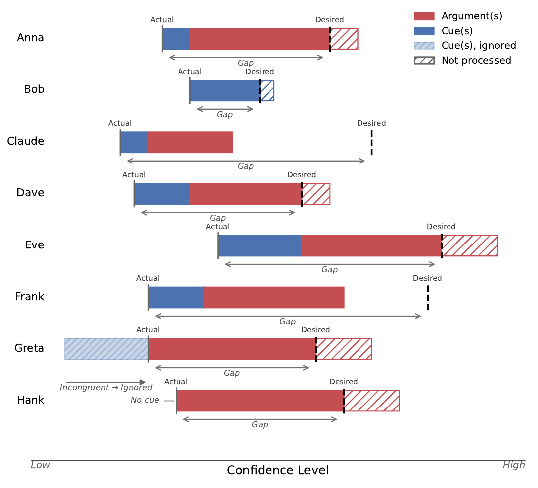
HSM is about someone who decides whether to draw a conclusion and act on it. Before looking at any information, the person has an Actual Confidence and a Desired Confidence (the Sufficiency Threshold). The distance between them is the gap. Information is processed with as little effort as possible: first the cues (heuristic processing, for example who says it), and only if the gap is still open the arguments (systematic processing). Processing stops as soon as the threshold is reached, and the person acts. If it is never reached, the person does not act.
Where the predictions come from
Nobody can measure these bars. The theory allows everybody to differ in where they start, where they want to get, and how strongly cues and arguments move them. All that is observed is whether a person acts. Two things still hold for every single person. A stronger argument never shortens the red bar, so anyone who acts with a weak argument also acts with a strong one. And a smaller gap never makes anybody stop acting. So in any population the share of people who act cannot fall when the argument gets stronger or the gap smaller. These are order constraints on proportions, exactly the kind of model the app handles.
Four probabilities and three predictions
The first study has two gap sizes (big b or small s) and two argument strengths (weak W or strong S). The four probabilities are the share of people who act in each condition, in this order: p1 = \(P_{bW}\) (big gap, weak argument), p2 = \(P_{bS}\), p3 = \(P_{sW}\), p4 = \(P_{sS}\).
p1 < p2; p3 < p4p1 < p3; p2 < p4p1 < p2 < p4; p1 < p3 < p4Vertices: the extreme cases
With Go and the V switch for m3, the app lists the six vertices of prediction 3. Each is a pattern across the four conditions: 1 means that everybody acts, 0 that nobody does. These are the extreme cases of the prediction.
| big gap, weak | big gap, strong | small gap, weak | small gap, strong | |
|---|---|---|---|---|
| V1 | 0 | 0 | 0 | 1 |
| V2 | 0 | 1 | 0 | 1 |
| V3 | 0 | 1 | 1 | 1 |
| V4 | 0 | 0 | 1 | 1 |
| V5 | 0 | 0 | 0 | 0 |
| V6 | 1 | 1 | 1 | 1 |
V5 is nobody acting, V6 everybody. V1 is only a small gap with a strong argument. The supplement checks each of the six patterns against the theory and finds that every one can be produced by a suitable population, so prediction 3 is a tight statement of what HSM implies. The H-representation contains no redundant constraint besides the automatic bounds.
How restrictive is it? Volumes and an intersection
A quarter of all possible families of four probabilities satisfy prediction 1, and a quarter prediction 2. Only one in twelve satisfy prediction 3. So with only four conditions the largest possible Bayes factor is already 12 for prediction 3 against the unconstrained model. This is the intersection of the first two: the Intersection model button gives for m1 and m2 the same volume, 1/12, as m3.
Replication: the same prediction in two populations
What if prediction 3 has to hold in two populations at once, for example women and men? The button Unpack across items repeats a model over items. With the base model m3 and two items:
- joint (item by item): the model holds in every population, eight probabilities. The volume is 1/144 and the largest possible Bayes factor 144.
- substitutable (all combinations of items): every probability of one population must also respect the order against the probabilities of the other, for example \(P_{bW}\) of one population is also at most \(P_{sW}\) of the other. The volume is 1/420, the largest possible Bayes factor 420.
Yet one richer study, with three gap sizes and three argument strengths (nine probabilities, twelve inequalities), reaches about 8,600 according to the supplement. So more conditions in a single study put far more pressure on the theory than the same small study replicated.
Cues: Override, Trade-off and Take-the-best
The second question asks what happens to the cues of a message: congruent with the conclusion (c), incongruent (i) or absent (n). Arguments are weak (W) or strong (S) as before; gap size is dropped. The six probabilities are, in this order: p1 = \(P_{iW}\), p2 = \(P_{nW}\), p3 = \(P_{cW}\), p4 = \(P_{iS}\), p5 = \(P_{nS}\), p6 = \(P_{cS}\).
\(P_{cS} \geq P_{cW} \geq P_{nW} = P_{iW}\) and \(P_{cS} \geq P_{iS} = P_{nS} \geq P_{nW}\)
p1 = p2 < p3 < p6; p2 < p4 = p5 < p6\(P_{cS} \geq P_{cW} \geq P_{nW} \geq P_{iW}\) and \(P_{cS} \geq P_{nS} \geq P_{iS} \geq P_{iW}\) and \(P_{nS} \geq P_{nW}\)
p1 < p2 < p3 < p6; p1 < p4 < p5 < p6; p2 < p5\(P_{iW} = P_{iS} = 0\) and \(P_{nW} = P_{nS} = P_{cW} = P_{cS} = 1\)
p1 = p4 = 0; p2 = p3 = p5 = p6 = 1What the app shows for the three models
- The Override model has two equalities and four inequalities. Its volume is zero, so there is no upper limit for the Bayes factor in its favour, and none against it. It has six vertices: nobody acts except with congruent cues and a strong argument (OH1), only people with congruent cues act whatever the argument (OH2), and so on up to everybody acting in every condition (OH6). Each can be produced by a suitable population.
- The Trade-off model has seven inequalities, ten vertices and a volume of 1/144: the largest possible Bayes factor is about 144. The Override model is nested in it.
- Take-the-best fixes every probability and therefore has exactly one vertex, the pattern (0, 1, 1, 0, 1, 1). It violates the Override model, since this pattern is not among the six vertices of Override. Because all its probabilities are fixed it has no volume: it is extremely restrictive and easy to falsify.
The six vertices of the Override model, as in Table A4 of the supplement (1 = everybody acts, 0 = nobody acts), and the single vertex of Take-the-best:
| incongruent, weak | no cues, weak | congruent, weak | incongruent, strong | no cues, strong | congruent, strong | |
|---|---|---|---|---|---|---|
| OH1 | 0 | 0 | 0 | 0 | 0 | 1 |
| OH2 | 0 | 0 | 1 | 0 | 0 | 1 |
| OH3 | 0 | 0 | 1 | 1 | 1 | 1 |
| OH4 | 0 | 0 | 0 | 1 | 1 | 1 |
| OH5 | 0 | 0 | 0 | 0 | 0 | 0 |
| OH6 | 1 | 1 | 1 | 1 | 1 | 1 |
| Take-the-best | 0 | 1 | 1 | 0 | 1 | 1 |
A mixture of Override and Take-the-best
Could a mixture, in which some people follow the Override model and the rest Take-the-best, protect HSM from falsification? Mathematically, the mixture is the set of all patterns that blend the two models: its vertices are the vertices of both, and everything in between belongs to it. The Mixture model button does this for m1 and m3. Its H-representation keeps an equality, \(P_{nW} + P_{iS} = P_{iW} + P_{nS}\), together with five inequalities, so its volume is zero too, and it is extremely restrictive and easy to falsify. Evidence in its favour has no theoretical limit with only six probabilities, and neither has evidence against it. Override and Take-the-best are nested in it. A mixture does not make a theory immune: it can still be refuted.
Where to go from here
From a verbal theory to a model you can test: the steps you now know.
- Say what must hold. Write the theory as statements about proportions, and ask what must be true for every single person or condition.
- Type the constraints. Chains such as
p1 > p2 > p3, constraints separated by a semicolon, sums with weights, equalities and tolerances. - Look at the model. The H-representation lists what it allows, the V-representation its extreme cases, and the polytope shows it.
- Measure how restrictive it is. The volume and the largest possible Bayes factor tell how much evidence the theory can earn and how much it risks; intersections show what theories share and which one is nested in which.
- Test it with data. Bayes factors, estimates and diagnostics in the app, and frequentist tests in QTEST (step by step here).
Next steps
- Try your own theory. Open the app and type it into the first model row. Share or save turns your input into a link, a QR code or a file, and every PDF of the app has a line that restores exactly your input.
- Take the tours. The cringe study repeats this guide step by step, and A real theory: the Heuristic-Systematic Model shows the same steps for a theory of the literature. Both can be done hands-on with Try it yourself.
- Test the theories in QTEST. The frequentist p values, the Bayesian p value and the convergence checks need the program QTEST. The page Analysis in QTEST walks through it with the same data and the first model of this guide.
- Download what you need. The files for QTEST and multinomineq, an R script that runs the analysis on your own computer, and a LaTeX file of the H-representation. The R package fairy reproduces the analyses of the article.
- Report what does not work. Use report a bug at the bottom of the app.
References
The article this app accompanies, and the literature cited in this guide.
Questions, ideas, bugs? Use report a bug at the bottom of the app, or the repository on GitHub (the icon in the toolbar above the app).
This page lists what changed in the app and in the R package fairy, newest first. Each entry says what you can now do, not only what was changed in the code. The app is updated continuously; the date at the bottom of the app shows when it was last changed.
first on GitHub
after the redesign
The app today in short: models are typed as constraints on probabilities; the app shows their H- and V-representations, plots the polytopes, computes volume-based parsimony, unpacks models across items, and runs the multinomineq analysis or exports files for multinomineq and QTEST. Everything you set can be downloaded as an R script, and the R package fairy reproduces the analyses of the paper.
6 November 2026
A new Guide tab
- The tab Guide walks through the cringe study from the first probabilities to a first analysis, with 26 short animations of what happens in the app, a contents list, the nine theories to copy (also as one link that opens the app with all of them), a chapter on reading the Bayesian results, a chapter on the Heuristic-Systematic Model of the online supplement, and the literature in the margin. It replaces the older tutorial; the step-by-step analysis in QTEST has its own page, Analysis in QTEST.
Two interactive tutorials in the app
- Take a tour > The cringe study enters everything for you, step by step, from three probabilities to nine theories, intersections, volumes and a first Bayesian analysis of data with multinomineq. Switch to Try it yourself to type it in yourself (with hints and feedback), turn on Extras for questions to predict, background notes and a progress bar, and set the speed with a control like in a video player (0.5x to 4x). Values a step talks about are framed in orange, and the card says what the frame shows.
- Take a tour > A real theory: the Heuristic-Systematic Model formalizes the textbook theory of the online supplement of the article: the figure of the theory, the order constraints that follow from it, volumes and largest possible Bayes factors (also for replications, using Unpack across items), the Override, Trade-off and Take-the-best models and a mixture of two of them.
Fixed
- The multinomineq analysis and the multinomineq download failed when a probability name contained a comma, such as p_{C,i}. They work now. If you downloaded files for such a model before, download them again.
5 November 2026
A guided tour
- Take a tour (top right of the app) explains the app step by step: each part is lit while the rest stays in the background. Choose the Start page for a first look, the Full tour for everything, or one part only: the input controls, the unpacking window, combining models (intersection, mixture), the result tabs, the run window, or the multinomineq analysis.
Share your input
- Link and QR code: Share or save > Share link or QR code of this input shows a QR code in the middle of the screen (with a tiny fairy hidden in it), copies the link, and saves the code as PDF or PNG.
- Every PDF of the app (multinomineq results, Parsimony, polytope, unpack picture) now has a clickable line Restore these models in the Fairy app that opens the app with exactly your input.
Unpack across items
- With several item lists, joint now pairs the items across lists item by item: item k of one list with item k of the other, and items without a partner are left out. Before, every item of one list was combined with every item of the other. Substitutable still uses all combinations. The picture, the statements and the R package follow the same rule, so results of such models change.
- The picture draws a sum of probabilities from different lists with one square per item, and compares rows of different lists item by item.
R package: fairy 0.6.6 on GitHub.
4 November 2026
From model to data analysis, all in the app
- Script download: On the Input page, under Download, you can download an R script with the commands for the package. Everything you set in the app is written into the script, so whatever you enter in the app can be reproduced with it.
- multinomineq files: On the H-representation page you can download the files for multinomineq (Heck’s R package), including a complete analysis script based on your models.
- Data entry in the app: Enter your observed counts (n and frequency) under Data; the data file in the right format is written for you. For unpacked models you can choose which model’s numbers they use.
- Analysis in the app (new): Run analysis runs the multinomineq analysis directly in the app. It is time-limited and meant for trying things out; for larger analyses, download the files and run the script on your own computer.
Volumes
- The exact volume is calculated first (corner points with rcdd, volume with geometry). It has a time limit and can be skipped; the algorithm only steps in when the exact volume was skipped or did not finish in time.
Unpack across items
- The diagram is drawn directly from the typed model (no Go needed first) and covers any linear constraint: sums, differences, weights, constants and chains.
Working with the app
- A big Go button (Input and Parsimony), with Share/Save and Upload next to it.
- The run windows give feedback while they work; skipping, cancelling and retrying work the same way everywhere.
- H-representation display: Parameters colours the terms by parameter (p1, p2 …), and Items marks the items of unpacked models with coloured bars. In both, single parameters or items can be deselected: the selected terms get a yellow marker and the rows can be filtered (all marked / some marked), also in expanded cards. Switching the parameter colour no longer moves the cards.
- All unpacked models now use the same default order of the probabilities (by probability, then by item), so the numbering p1, p2 … in the downloads is the same for all of them.
- A calmer look of all windows, a Compact layout with one line per model, and controls for the embedded app (new session, unload, Fill window / full screen).
- Many smaller fixes and refinements.
R package: fairy 0.6.5 on GitHub.
2 - 3 November 2026: windows, plots and the unpack picture
- The unpack picture draws sums, differences, weights and constants, and warns about non-linear input; the 3D polytope can be saved as a vector PDF.
- Skipping and retrying a calculation work per model in every run window, and Fill window of the embedded app gets its own exit button.
- The multinomineq results come as a PDF; Compare only offers models that live in the same space.
- R package fairy 0.6.
1 November 2026: exact volumes and multinomineq
- The exact volume runs as a background job with progress and a time limit; Parsimony has separate switches for the exact volume and the algorithms.
- Cancel is the one verb for stopping a calculation.
- multinomineq in the app: choice of the number of samples, data entry, and results with the strength of evidence in colour.
- Plot Edge Cases gets an overview and lists all vertices in blocks.
29 - 31 October 2026: order of the probabilities
- The order of the probabilities of an unpacked model can be changed by dragging; it holds for QTEST, multinomineq and the exported script.
- The unpack dialog was redesigned (one settings row, short options); its picture can be saved as a PDF.
- Mixtures and intersections keep the shape of deleted source models; the tolerance dialog names the equalities that force a pair.
28 October 2026: R package 0.4 and 0.5
- fairy 0.4: volesti defaults and no automatic switch of the volume method. fairy 0.5: model tables, a readable H-table and writers for QTEST and multinomineq.
- The exported R script has a seed, clearer comments and tables per model; the embedded app can be opened alone in a new tab with the current input.
25 - 27 October 2026: the picture for unpacking
- Several item sets per model (own group and count per set), a preview of the generated statements, and a picture that shows which items are compared; the weights of sums are shown.
- The V tab shows the counts of shared and unique vertices.
24 October 2026: sharing and the R package
- Share links restore an input; a Share/Save menu and keyboard help were added.
- The R package fairy was added; it reproduces the analyses of the paper and its supplement, with vignettes.
22 - 23 October 2026: one window for all calculations
- A quiet loading screen, and one persistent run window with progress for all models and both representations.
- Model cards in the H- and V-representation tabs can be re-ordered by dragging their title.
1 October 2026: major update
- A redesign of the whole interface: dark mode, a compact layout, tooltips, accessibility (keyboard use, contrast, labels) and cleaner exports (QTEST, multinomineq, LaTeX).
September 2024 - March 2025: the app as fairy
- The app continued under its current name in the current repository: models as constraints on probabilities, their H- and V-representations, plots of the polytopes and volume-based parsimony.
November 2022 - May 2024: gui_qtest
- The first Shiny version, kept in an earlier repository (gui_qtest) before the app moved to its current one: models typed as constraints, H- and V-representations (rcdd), plots, and volumes (volesti).
This overview was written with the help of AI (Claude, by Anthropic) from the commit history of the project, and reviewed by Marc Jekel.